
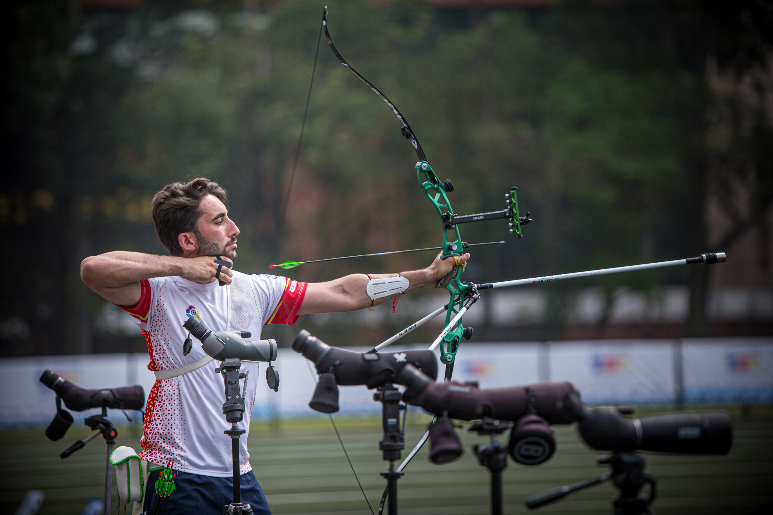
In the third of a series of articles, Dr James Park looks at what we can learn studying the dynamic behaviour of arrows during the power stroke and in-flight
In Bow 156, I noted that while I use X10s, size 600, with my recurve bow for target archery – because I want the least wind drift – I also wanted a lower mass arrow for field archery. After some careful modelling, I selected ACEs, size 670, as I was confident that I would be able to use them with the same draw force, changing just the pressure button at most.
In Bow 157, I provided an overview of how I model arrows. I consider them as inextensible, flexible beams consisting of many short sections joined together. Each of those sections has its diameter, mass and stiffness. I showed how I determine those parameters for each arrow type and size.
In this article I will provide an overview of how that modelling can be used to study the arrow’s dynamic behaviour during the bow’s power stroke and then in free flight.
The first interesting paper in this area was by Pekalski in 1990. Kooi then made a major step forward in his paper on the archer’s paradox in 1997. In both those cases, they considered tubular aluminium arrows shot from a recurve bow. Kooi’s results were impressive.
I used a technique similar to that used by Kooi, but extended it to cover tapered and barrelled carbon/aluminium arrows and also considered arrows in free flight.
Each small segment of the arrow shaft can be modelled as an inextensible, flexible beam, with additional masses added at the appropriate locations for the nock, fletching and point as described in my previous article. The point shank slightly changes the stiffness of the front segments of the arrow.
The beam segments are each subject to the Euler-Bernoulli beam equation (where EI is the stiffness) and to Newton’s second law of motion:
External forces
There are also some external forces acting on the arrow. These include the force from the bow’s string, the force from the bow’s pressure button or launcher, gravity and aerodynamic drag and lift. It is also necessary to have a mathematical model for the pressure button or launcher.
Together, the beam equation and Newton’s second law give us either a fourth-order or two simultaneous second-order partial differential equations (in time and space), which describe the arrow’s flex. The boundary conditions are moving and non-linear. The position of the arrow along the line towards the target also needs to be calculated using Newton’s second law. This will probably look a bit daunting to most non-engineers or non-mathematicians, but they are in fact reasonably amenable to solution.
Certainly, if you are not familiar with this sort of thing, the mathematics in Kooi’s or my papers might look a little challenging. I may be biased, but I suspect my paper might be a little easier to follow. Kooi provides more general-difference equations covering each of the three finite difference methods while I cover one of those, and mine provides a little more explanation.
Kooi and I both solved the equations using finite difference methods. This can be implemented quite easily in Excel, although that is not as flexible as a purpose-built application. I first implemented it in Excel and then, when I knew it was working, created my analysis programs.
I now have applications covering arrow behaviour in recurve bows (for both the horizontal and vertical planes), compound bows and in free flight. If you want to try implementing a similar application, a good place to start would be the difference equations in my paper.
It is necessary to understand how the string leaves an archer’s fingers when using a recurve bow. To achieve that, I studied many high-frame-rate videos kindly provided in Archery GB after the London 2012 test event. The top recurve archers all have the string leave their middle finger last. I measured the lateral and longitudinal displacement of the string as it came off the finger tab for each archer and used that in my modelling.
It is also necessary to have a model of the force of the string pushing on the arrow. This is the bow’s dynamic force-draw curve, not the static force-draw curve (which is the force you need to exert in drawing the bow). This is not easy to calculate. One approach would be to use the model in Kooi’s paper. The dynamic force-draw differs from the static force-draw curve because, as well as accelerating the arrow during the bow’s power stroke, the mass of the limbs and string needs to be accelerated.
Then, late in the power stroke, the kinetic energy of the limbs is (mostly) given to the arrow. A good way to manage the uncertainty in the modelling in this area is to measure the exit arrow speed of an arrow of known mass and to adjust the dynamic force-draw model to give that arrow speed.
If you wish to include the aerodynamic drag and lift forces on the arrow, the easiest approach would be to use the methods in my papers. However, during the bow’s power stroke, it is reasonable to ignore them. You do need to include them when considering the arrow in free flight.
If you are considering arrow behaviour in the vertical plane, you do need to allow for the arrow flexing under gravity while it is at full draw in the bow prior to release.
Putting it together
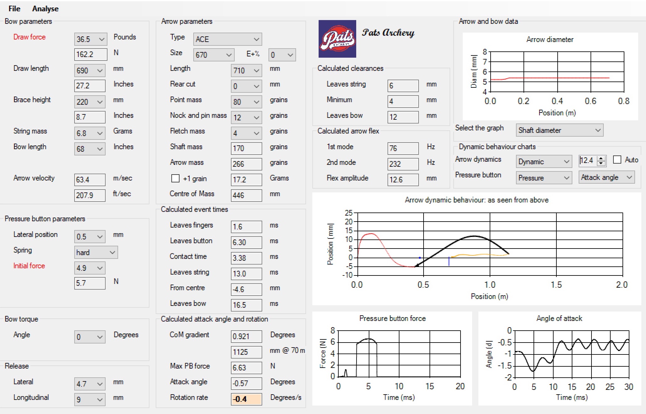
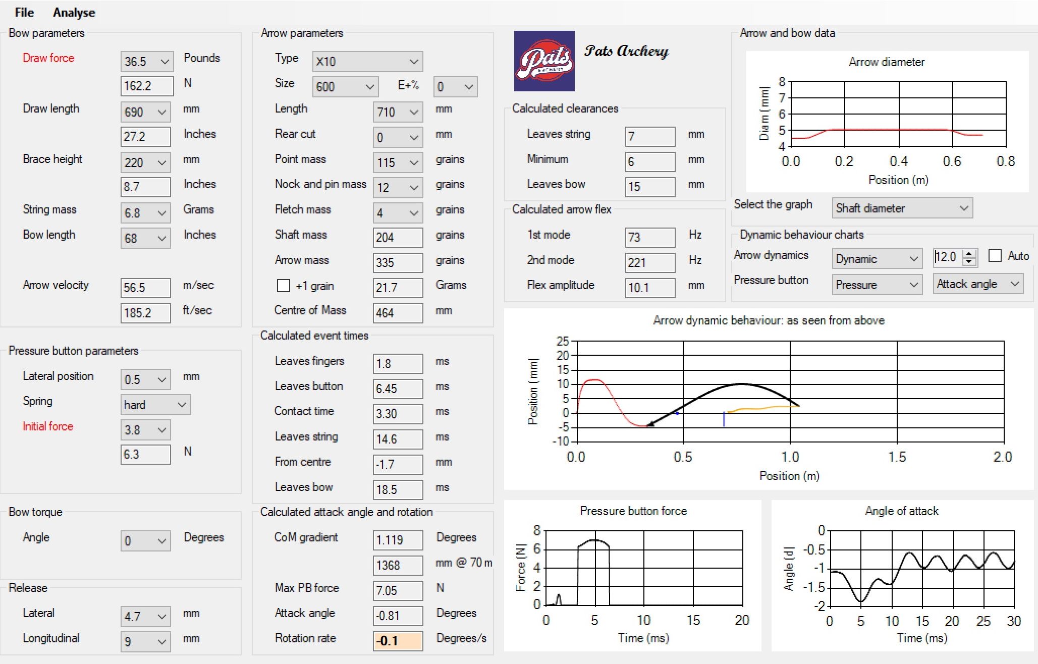
Having the models mentioned above, I first modelled my X10s, size 600, exiting my recurve bow. I knew they tuned well, and I had measured their speed and mass. Hence, I knew their orientation, lateral rotation and flex as they left the bow. In addition, I checked the calculated arrow flex photographically. (The picture below shows it for a previous bow and a set of X10s.)
I wanted the lowest mass, small-diameter arrow that would tune the same as the X10s. Hence, I looked at how ACE’s, sizes 620 and 670 were likely to behave. The 670s appeared more attractive due to their lower shaft mass. I could get both to tune nicely, but to do so the 670s needed a much lower point mass than the 620s, which would also give a lower overall shaft mass. Having run my models, I bought the shafts; everything worked as expected.
In the end, I have the following:
For target archery: X10, size 600, 115 grain point, spin wings, 710mm shaft, mass of 335 grains, 185ft/sec.
For field archery: ACE size 670, 80 grain point, spin wings, 710mm shaft, 266 grains, 208ft/sec.
That is a nice gain of 23ft/sec for field archery. And with an arrow that has a reasonably small diameter and hence will be reasonable when it is windy (although not as good as the X10s when it is windy).
Above are two screen shots from my modelling, one for the X10s and the other for the ACEs. Aside from the arrows, you can see that all I have changed is to make the pressure button pressure just a tiny bit less for the ACEs than for the X10s.
We want the arrow to exit the bow in line with its direction of travel and with close-to-zero longitudinal rotation about its centre of mass (the highlighted parameter near the bottom of each picture). The angle of attack is shown in the chart on the bottom right. If the arrow is aligned as desired, the plot will be horizontal after the arrow has left the string (and it is in both cases). The ripple is a consequence of flexes higher than the first mode, which is OK – and expected.